
Linear Discriminant Analysis#
Author: Nathan A. Mahynski
Date: 2023/09/12
Description: Derivation and examples of LDA. LDA is similar to PCA in that it tries to find the linear combination of features that characterize, or summarize, the data; however, unlike PCA, LDA explicitly attempts to model the differences between classes (supervised) rather than just the “shape” of the data (unsupervised) like PCA does.
A thorough comparison discriminant analysis methods can be found at All Models are Wrong or Sebastian Raschka’s blog. LDA is a supervised method that can be used for classification or dimensionality reduction (often followed by classification).

[ ]:
if 'google.colab' in str(get_ipython()):
    !pip install git+https://github.com/mahynski/pychemauth@main
    import os
    os.kill(os.getpid(), 9) # Automatically restart the runtime to reload libraries
[ ]:
try:
    import pychemauth
except:
    raise ImportError("pychemauth not installed")

import matplotlib.pyplot as plt
%matplotlib inline

import watermark
%load_ext watermark

%load_ext autoreload
%autoreload 2
[ ]:
import sklearn
import imblearn

import numpy as np

from imblearn.pipeline import Pipeline
from sklearn.preprocessing import LabelEncoder
from sklearn.datasets import make_blobs
from sklearn.discriminant_analysis import LinearDiscriminantAnalysis as LDA
from sklearn.inspection import DecisionBoundaryDisplay
from sklearn.model_selection import train_test_split, GridSearchCV, StratifiedKFold
from sklearn.linear_model import LogisticRegression

from pychemauth.preprocessing.scaling import CorrectedScaler
[ ]:
%watermark -t -m -v --iversions
Python implementation: CPython
Python version       : 3.10.12
IPython version      : 7.34.0

Compiler    : GCC 11.4.0
OS          : Linux
Release     : 6.1.85+
Machine     : x86_64
Processor   : x86_64
CPU cores   : 2
Architecture: 64bit

matplotlib: 3.7.2
watermark : 2.4.3
pychemauth: 0.0.0b4
imblearn  : 0.11.0
numpy     : 1.24.3
sklearn   : 1.3.0
LDA as a classifier#
LDA classifiers are attractive because they:
Have closed-form solutions that can be easily computed,
Are inherently multiclass, have proven to work well in practice,
Have no hyperparameters to tune!
However, LDA makes certain strong assumptions when functioning as a classifier:
The data is normally distributed,
The features are statistically independent,
Covariance matrices are identical for every class.
Why is that? LDA can actually be derived from probabilistic models that describe the class conditional distribution of the data, namely \(P(y=k|x)\), for class \(k\) given \(x\). LDA assigns a point to the class whose mean is closest in terms of Mahalanobis distance while also accounting for the class prior probabilities.
scikit-learn discusses this here, and more details can be found in Hastie et al. “The Elements of Statistical Learning” (2008).
From Bayes’ Law we have (note this assumes \(x\) is a row vector; if column format is used the transposes below will switch around):
The denominator is a constant which can be disregarded. In LDA (and QDA) one simply chooses to model \(P(x|y)\) as a multivariate Gaussian as follows:
where \(\Sigma_k\) is the covariance matrix of class \(k\) and \(\mu_k\) is mean vector of class \(k\); \(d\) is the original dimensionality of \(x\). The argument of the exponent is the Mahalanobis distance. QDA uses the covariance matrices of each class, however, if we assume they are the same (homoscedasticity assumption), then we can write:
Using the fact that the covariance matrix is Hermitian, this can be simplified to:
We are looking for the smallest distance, or maximum \({\rm ln}P(y=k|x)\), across all classes; note the first term in the Mahalanobis distance expansion does not depend on \(k\) so it is constant value across all \(k\) expressions. Thus, we can write:
where \(C''\) absorbs the constants from the Gaussian, denominator in Bayes’ Law, and first term in the Mahalanobis distance expansion. This can be rewritten as:
where \(\omega_k = \Sigma^{-1}\mu_k^T\) and \(\omega_{k,0} = -\frac{1}{2}\mu_k \Sigma^{-1} \mu_k^T + {\rm ln}P(y=k)\) (in practice the \(C''\) is neglected). sklearn stores theses as coef_ and intercept_ in the LDA object. The linear nature of this equation is why it is known as “linear” DA, vs. when we make no assumptions about \(\Sigma_k\) being equal for all classes, the result is quadratic (because the first term in the Mahalanobis distance expansion must be retained
since it depends on \(k\) now), hence QDA.
Consequently, the above decision function can be computed (see sklearn.discrimininant_analysis.LinearDiscriminantAnalysis.decision_function) to provide the log probability of a given class. Normalizing over all classes gives the sklearn.discrimininant_analysis.LinearDiscriminantAnalysis.predict_proba result, or the ability to predict the class probability.
Estimating the covariance matrix#
The assumption in LDA is that the covariance matrix is the same for each class, but how do we actually estimate this from our data? In practice, this is done by a (de-biased) weighted average (i.e., the pooled variance) of each class’ covariance matrix.
See this stackexchange question. Note that sklearn can accommodate other estimation methods, though.
Implement the Algorithm
[ ]:
def lda_ln_prob(X_test, X_train, y_train):
    """Compute the lnP of classes based on LDA model of data."""

    # Assume that we are comparing to LDA using pre-scaled data
    scaler = CorrectedScaler(with_mean=True, with_std=True)
    X_train = scaler.fit_transform(X_train)

    # Encode classes an integers and transform
    enc = LabelEncoder()
    y_train = enc.fit_transform(y_train.ravel())

    # Identify the empirical means for each class
    means = {}
    for c in [enc.transform([class_])[0] for class_ in enc.classes_]:
        mask = y_train == enc.inverse_transform([c])[0]
        means[c] = np.mean(X_train[mask], axis=0)

    # Compute pooled covariance estimate
    sigma = np.zeros((X_train.shape[1], X_train.shape[1]))
    for c in [enc.transform([class_])[0] for class_ in enc.classes_]:
        mask = y_train == enc.inverse_transform([c])[0]
        N = np.sum(mask)
        sigma += (N-1)*np.cov(X_train[mask].T)
    sigma /= (X_train.shape[0] - len(np.unique(y_train)))

    # lda.coef_
    coef = []
    for c in [enc.transform([class_])[0] for class_ in enc.classes_]:
        coef.append(np.matmul(np.linalg.inv(sigma), means[c].T))

    # lda.intercept_
    intercept = []
    for c in [enc.transform([class_])[0] for class_ in enc.classes_]:
        intercept.append(-0.5*np.matmul(np.matmul(means[c], np.linalg.inv(sigma)), means[c].T)+np.log(np.sum(y_train==enc.inverse_transform([c])[0])/X_train.shape[0]))

    # Predict on test set
    d = X_train.shape[1]
    probs = np.zeros((X_test.shape[0], len(enc.classes_)))
    for i,x in enumerate(scaler.transform(X_test)):
        for j in [enc.transform([class_])[0] for class_ in enc.classes_]:
            probs[i,j] = np.dot(coef[j], x) + intercept[j] # Constants related to Gaussian prefactor are ignored in sklearn

    return probs, coef, intercept
[ ]:
# Let's make some sample data
X, Y = sklearn.datasets.make_blobs(
    n_samples=100,
    n_features=2,
    centers=3,
    cluster_std=.5,
    shuffle=True,
    random_state=0
)
[ ]:
for class_ in np.unique(Y):
    X_ = X[Y == class_]
    plt.scatter(X_[:,0], X_[:,1], label=f'Class {class_}')
plt.legend(loc='best')
plt.xlabel(r'$X_1$')
_ = plt.ylabel(r'$X_2$')

[ ]:
# For this example we will use the entire dataset for training
scaler = CorrectedScaler()
lda = LDA(n_components=1, store_covariance=True)
_ = lda.fit(scaler.fit_transform(X), Y)
[ ]:
my_ln_probs, coef, intercept = lda_ln_prob(X, X, Y.reshape(-1,1))
sklearn_ln_probs = lda.decision_function(scaler.transform(X))

# To prevent overflow
my_shifted_probas = (my_ln_probs.T - np.max(my_ln_probs, axis=1)).T

my_probas = (np.exp(my_shifted_probas).T/np.sum(np.exp(my_shifted_probas), axis=1)).T
sklearn_probas = lda.predict_proba(scaler.transform(X))
[ ]:
assert np.allclose(my_ln_probs, sklearn_ln_probs) # Manual decision function agrees with sklearn
assert np.allclose(my_probas, sklearn_probas) # Manual class probability agrees with sklearn
assert np.allclose(lda.coef_, coef) # Manual coef agrees with sklearn
assert np.allclose(lda.intercept_, intercept) # Manual intercept agrees with sklearn
[ ]:
disp = DecisionBoundaryDisplay.from_estimator(lda, scaler.transform(X))

for class_ in np.unique(Y):
    X_ = scaler.transform(X)[Y == class_]
    disp.ax_.scatter(X_[:,0], X_[:,1], label=f'Class {class_}')
disp.ax_.legend(loc='best')
disp.ax_.set_xlabel(r'$X_1$')
_ = disp.ax_.set_ylabel(r'$X_2$')

Impact of Class Imbalance
Observe that the constant in the discriminant function involves a term \({\rm ln}P(y=k)\). This comes from the prior in the first equation (Bayes’ Law). This is absorbed in the intercept_ and may be relative weak compared to other terms, but it is nonetheless a factor in determining the boundary.
[ ]:
def make_imblance(factor=10):
    X, Y = sklearn.datasets.make_blobs(
        n_samples=500,
        n_features=2,
        centers=2,
        cluster_std=1,
        shuffle=True,
        random_state=0
    )

    # Let's remove a fraction of class 0 relative to the others
    mask = Y == 0

    X_ = X[~mask]
    Y_ = Y[~mask]

    X_ = np.vstack((X_, X[mask][:np.sum(mask)//factor]))
    Y_ = np.concatenate((Y_, Y[mask][:np.sum(mask)//factor]))

    return X_, Y_

def visualize(lda, scaler, X, Y, ax):
    disp = DecisionBoundaryDisplay.from_estimator(lda, X, ax=ax, response_method='predict')

    for class_ in np.unique(Y):
        X_ = X[Y == class_]
        disp.ax_.scatter(X_[:,0], X_[:,1], label=f'Class {class_}')
    disp.ax_.legend(loc='best')
    disp.ax_.set_xlabel(r'$X_1$')
    disp.ax_.set_ylabel(r'$X_2$')
    disp.ax_.set_xlim(-1.5, 5)
[ ]:
fig, axes = plt.subplots(nrows=1, ncols=2, figsize=(12,4))

# Balanced
X_, Y_ = make_imblance(factor=1)
scaler = CorrectedScaler()
lda = LDA(n_components=1, store_covariance=True)
_ = lda.fit(X_, Y_)

visualize(lda, scaler, X_, Y_, ax=axes[0])

# Imbalanced
X_, Y_ = make_imblance(factor=10)
scaler = CorrectedScaler()
lda = LDA(n_components=1, store_covariance=True)
_ = lda.fit(X_, Y_)

visualize(lda, scaler, X_, Y_, ax=axes[1])

LDA as a dimensionality reduction technique#
Interestingly, the LDA model also can function as a dimensionality reduction tool. In fact, this is how it was originally derived by Sir Ronald Fisher in 1936 in a slightly form often called “Fisher’s linear discriminant.” Today, the terms are used interchangeably.
If 2 classes have means, \(\mu_0\) and \(\mu_1\), and covariances, \(\Sigma_0\) and \(\Sigma_1\), then the linear combination of features \(\vec{w} \cdot \vec{x}\) will have mean \(\vec{w} \cdot \mu_i\) and variance \(\vec{w} \Sigma_i \vec{w}^T\) for each class, \(i\). Fisher defined the separation between these distributions as the ratio of the variance between the classes to the variance within the classes:
Maximum separation occurs when:
When classes are normally distributed and have equal covariances (LDA classifier assumptions) this results in the same equations above.
According to Wikipedia:
“Linear discriminant analysis (LDA), normal discriminant analysis (NDA), or discriminant function analysis is a generalization of Fisher’s linear discriminant, a method used in statistics and other fields, to find a linear combination of features that characterizes or separates two or more classes of objects or events. The resulting combination may be used as a linear classifier, or, more commonly, for dimensionality reduction before later classification. “
Sebastian Raschka has a nice discussion here with illustrations in python.
“It should be mentioned that LDA assumes normal distributed data, features that are statistically independent, and identical covariance matrices for every class. However, this only applies for LDA as classifier and LDA for dimensionality reduction can also work reasonably well if those assumptions are violated.”
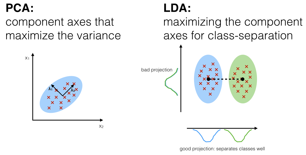
With PCA, we found the orthogonal principal components that characterized the spread of the data, i.e., the covariance of X with itself (unsupervised). With PLS, we looked for directions that characterized the covariance of the product of X and Y (supervised). LDA is a supervised method which instead looks for axes that maximize the separation between labelled classes. This is done by finding the eigenvectors (“linear discriminants”) of the matrix \(S_W^{-1}S_B\), where \(S_W\) is the within-class scatter matrix and \(S_B\) is the between-class scatter matrix. LDA for dimensionality reduction can be described in 5 steps:
Compute the \(p\)-dimensional mean vectors for all classes from the dataset.
Compute the scatter matrices (between-class and within-class scatter matrix).
Compute the eigenvectors and eigenvalues for these matrices.
Sort the eigenvectors by decreasing eigenvalue and choose the first \(k\) eigenvectors; stack these columns to form a \(p \times k\) dimensional matrix \(W\). This is analogous to the “loadings” matrix in PCA.
Use this \(p \times k\) matrix to project the samples into the new subspace by performing matrix multiplication: \(T = XW\), where \(T\) are the “x-scores”.
PCA can be used to perform dimensionality reduction by only selecting the leading \(k\) eigenvectors from the covariance matrix; assuming it is full rank, we have as many dimensions as the size of that matrix. However, in LDA, the matrix \(S_W^{-1}S_B\) will only have at most \({\rm min}(p, c-1)\) non-zero eigenvectors where \(p\) is the number of features and \(c\) is the number of classes. Thus, if we want to separate 2 classes, LDA will only be able to return the single axes that separates them best. In such a case, it might be better to even do PCA if we desire a low, but higher than 1-, dimensional result.
In general though, the intuitive explanation for LDA is that it finds the orthogonal axes that best separate classes. Thus, it is a very useful dimensionality reduction approach for classification. It is particularly helpful in identifying a subspace that is highly discriminative, in which other models can be used to compute decision boundaries. For example, a pipeline might look like:
Standardize data
LDA to project into a small number of dimensions
Use logistic regression to classify
[ ]:
data = sklearn.datasets.load_iris()
X = data.data
y = data.target
X_train, X_test, y_train, y_test = train_test_split(X, y, stratify=y, shuffle=True, train_size=0.8, random_state=0)
[ ]:
# Scale and perform LDA to project into 2D
scaler = CorrectedScaler()
lda = LDA(n_components=2)
X_train_std_lda = lda.fit_transform(scaler.fit_transform(X_train), y_train)
[ ]:
# In LDA this is called the "discriminability" ratio and is the ratio of the
# eigenvalues, just like in PCA
lda.explained_variance_ratio_
array([0.98972886, 0.01027114])
[ ]:
# Compare this to PCA in the same number of dimensions
from sklearn.decomposition import PCA
pca = PCA(n_components=2).fit(scaler.transform(X_train))
pca.explained_variance_ratio_
array([0.72716189, 0.23524787])
[ ]:
# The "transform" member does the matrix multiplication to obtain the scores
np.allclose(
    X_train_std_lda,
    np.matmul(scaler.transform(X_train), lda.scalings_)
)
True
[ ]:
# The "W" matrix is stored as the "scalings_" member of the LDA object.
# Recall, these are the coefficients on each feature for each eigenvector
# we have computed.

lda.scalings_
array([[ 0.82232406, -0.56359583],
       [ 0.57264111, -0.78635556],
       [-3.68399263,  2.3632896 ],
       [-2.26007987, -2.31926631]])
[ ]:
# Here is the analogy in PCA.  Clearly these two methods have found different
# vectors which "summarize" the data!
pca.components_.T
array([[ 0.52798835,  0.35662823],
       [-0.24446693,  0.9326461 ],
       [ 0.5819892 ,  0.01776533],
       [ 0.56811336,  0.05169099]])
[ ]:
# We can build the analogy of a loadings plot in PCA by using the scalings.
# This allows to interpret which features are the most significant in terms
# of what features SEPARATE the classes.

fig, axes = plt.subplots(nrows=1, ncols=2, figsize=(12,4))

for name, pos in zip(data['feature_names'], lda.scalings_):
    axes[0].plot(pos[0], pos[1], 'o', color='C0', label=name)
    axes[0].text(pos[0], pos[1], name)
axes[0].axvline(0, ls='--', color='k')
axes[0].axhline(0, ls='--', color='k')

axes[0].set_xlabel(f'LD 1 ({"%.3f"%(lda.explained_variance_ratio_[0]*100)}%)')
axes[0].set_ylabel(f'LD 2 ({"%.3f"%(lda.explained_variance_ratio_[1]*100)}%)')
axes[0].set_title('LDA')

for name, pos in zip(data['feature_names'], pca.components_.T):
    axes[1].plot(pos[0], pos[1], 'o', color='C0', label=name)
    axes[1].text(pos[0], pos[1], name)
axes[1].axvline(0, ls='--', color='k')
axes[1].axhline(0, ls='--', color='k')

axes[1].set_xlabel(f'PC 1 ({"%.3f"%(pca.explained_variance_ratio_[0]*100)}%)')
axes[1].set_ylabel(f'PC 2 ({"%.3f"%(pca.explained_variance_ratio_[1]*100)}%)')
axes[1].set_title('PCA')
Text(0.5, 1.0, 'PCA')

[ ]:
# Train a LR classifier in LDA's 2D space
lr = LogisticRegression(C=1.0, random_state=0)
_ = lr.fit(X_train_std_lda, y_train)
[ ]:
disp = DecisionBoundaryDisplay.from_estimator(lr, X_train_std_lda, response_method='predict', grid_resolution=1000)

for class_ in np.unique(y_train):
    X_ = X_train_std_lda[y_train == class_]
    disp.ax_.scatter(X_[:,0], X_[:,1], label=f'Class {class_}')
disp.ax_.legend(loc='best')
disp.ax_.set_xlabel(r'LD 1')
disp.ax_.set_ylabel(r'LD 2')
Text(0, 0.5, 'LD 2')

You can see that the decision boundaries along the first component axis (x-axis) are nearly vertical - this is because LDA finds the axes that best separate the classes from each other as you move along it. The data here is particularly amenable to this approach.
[ ]:
pipe = Pipeline([
    ('scaler', CorrectedScaler()),
    ('lda', LDA()),
    ('lr', LogisticRegression(random_state=0))
]
)

grid = [
    {'lda__n_components':[1,2], # Limited to n_classes-1
     'lr__C':np.logspace(-5,0,10),
    }
]

gs = GridSearchCV(
    estimator=pipe,
    param_grid=grid,
    refit=True,
    cv=StratifiedKFold(n_splits=10, shuffle=True, random_state=0),
    n_jobs=-1
)
_ = gs.fit(X_train, y_train)
[ ]:
gs.best_params_
{'lda__n_components': 2, 'lr__C': 0.2782559402207126}
[ ]:
gs.score(X_test, y_test)
1.0